Querying with Access Patterns and Integrity Constraints

Environments

We used the Amazon Web Services Elastic Cloud Computing platform running a Linux Operating system m3.xlarge instances. The details of the hardware and software used are the following:

Hardware		Software
Physical processor	Intel Xeon E5-2670 v2	Operating system	Amazon Linux (3.4.68-59.97.amzn1.x86_64)
Virtual CPUs	4	Java Runtime	OpenJDK 64-Bit Server VM (24.51-b03)
Clock speed (GHz)	2.5	DBMS (data storage)	PostgreSQL 9.2.7
Memory (GB)	15	DBMS (used internally by the planner)	MySQL 14.14, Distrib 5.5.34 (optional) if not available, the reasoner will fallback to an in-memory Derby-10.10 database instance, with lower performance
Storage (GB)	2 x 40 SSD
Network performance	High

Repeatability

The required software to reproduce the experiments has been packaged in a single JAR available here. For more details on how to run the program, type the following command in your favourite console:

java -jar /path/to/jar --help

Input parameters for the program can be passed in command line or specified in some external file (example). If you would like to use the sources, please contact the authors.

Cost model

The cost function used throughout these experiments is a basic ``textbook'' cost function. The cost is computed recursively starting the plan's root operator. Each operator computes its cost as the sum of the cost of its children, plus a local cost.

The computation of the local cost varies for each operator, and typically relies on the estimated cardinality of its inputs, of its output, that of its children's outputs, the width of the tuple handled, and the amount of "work" that needs to be done on those tuples. For instance, the cost of a selection is proportional to the size of its condition. The cost of each join algorithm variant is based on their respective complexity.

For cardinality estimation, we use a very simple approach, where the output of a join is computed as the upper bound (size of the cartesian product), divided by a constant factor (10). To mititage the propagation of errors, and since we assume our query all relies on join between key/foreign key attributes, we limited the size of the output to the size of the largest child.

In this experimental scenario, all our relations lie in a PostgreSQL DBMS, and the cost of independent accesses is obtained directly from the database. For each available access method, we bind arbitrary values to the required inputs, and send a corresponding query to the databases. This method allows us to account to the existing indices in the cost of individual accesses.

Schemata

The dataset used in the experiments is TPCH. We generated data using scale factors .001.

We conducted experiments using three schemas, all extending the standard TPCH schema with different sets of access restrictions and materialized views.

S_default features (i) three materialized views with free access and limited access methods for each indices, (ii) three free access relations (region, part, supplier), and (iii) five relations with limited access where input attributes correspond to foreign keys. These access methods ensure all our queries are anserwable. download

S_CP (cross product-oriented schema) only differs from S_default in its access restrictions. Required inputs are placed such as to limit the existence of cross product-free left-deep plans (15 of our 20 queries do not have any cross product-free left-deep plan with this schema). download

S_views (view-oriented schema) We used a schema featuring 12 views with free access and made the base relation inaccessible except region, nation and supplier. All queries are answerable using the accessible tables: we first added materialized views for every pair connected by a key-foreign key constraint, and then added one view for every triple of relations for which there exists a single "hub" relation having key-foreign key constraints with the two other relations, with the remaining relations not being associated via a key foreign-key dependency. download

Tables

• region

  Attribute name	Attribute Type
  r_regionkey	integer
  r_name	string
  r_comment	string
  Required inputs	Used in
  FREE	Sdefault, SCP, Sviews

• nation

  Attribute name	Attribute Type
  n_nationkey	integer
  n_name	string
  n_regionkey	integer (@region.r_regionkey)
  n_comment	string
  Required inputs	Used in
  FREE	Sview
  3	Sdefault, SCP

• customer

  Attribute name	Attribute Type
  c_custkey	integer
  c_name	string
  c_address	string
  c_nationkey	integer (@nation.n_nationkey)
  c_phone	string
  c_acctbal	double
  c_mktsegment	string
  c_comment	string
  Required inputs	Used in
  4	Sdefault
  1	SCP

• supplier

  Attribute name	Attribute Type
  s_suppkey	integer
  s_name	string
  s_address	string
  s_nationkey	integer (@nation.n_nationkey)
  s_phone	string
  s_acctbal	double
  s_comment	string
  Required inputs	Used in
  FREE	Sdefault, SCP, Sviews
  4	Sdefault
  2	SCP

• part

  Attribute name	Attribute Type
  p_partkey	integer
  p_name	string
  p_mfgr	string
  p_brand	string
  p_type	string
  p_size	integer
  p_container	string
  p_retailprice	double
  p_comment	string
  Required inputs	Used in
  FREE	Sdefault, SCP

• partsupp

  Attribute name	Attribute Type
  ps_partkey	integer (@part.p_partkey)
  ps_suppkey	integer (@supplier.s_suppkey)
  ps_availqty	integer
  ps_supplycost	double
  ps_comment	string
  Required inputs	Used in
  1	Sdefault
  2	Sdefault
  1,2	Sdefault, SCP

• orders

  Attribute name	Attribute Type
  o_orderkey	integer
  o_custkey	integer (@customer.c_custkey)
  o_orderstatus	string
  o_totalprice	double
  o_orderdate	date
  o_orderpriority	string
  o_clerk	string
  o_shippriority	integer
  o_comment	string
  Required inputs	Used in
  1	SCP
  2	Sdefault
  6	SCP

• lineitem

  Attribute name	Attribute Type
  l_orderkey	integer (@orders.o_orderkey)
  l_partkey	integer (@partsupp.ps_partkey)
  l_suppkey	integer (@partsupp.ps_suppkey)
  l_linenumber	integer
  l_quantity	double
  l_extendedprice	double
  l_discount	double
  l_tax	double
  l_returnflag	string
  l_linestatus	string
  l_shipdate	date
  l_commitdate	date
  l_receiptdate	date
  l_shipinstruct	string
  l_shipmode	string
  l_comment	string
  Required inputs	Used in
  2	Sdefault
  3	Sdefault
  1,2	SCP
  2,3	Sdefault, SCP

Materialized views

• region_nation (S_default, S_CP)

  SELECT n.n_nationkey as nation_key, n_name as nation_name,
         r.r_regionkey as region_key, r_name as region_name
  FROM nation as n, region as r
  WHERE n.n_regionkey = r.r_regionkey
  		    

  Access method name	Required inputs
  FREE	Sdefault, Sviews
  1	Sdefault
  2	SCP
  4	SCP

• order_supplier (S_default, S_CP)

  SELECT s.s_name as sname,
         s.s_address as saddress, s.s_nationkey as snation, 
         s.s_acctbal as sactbal, o.o_orderpriority as opriority,
         o.o_clerk as oclerk, p.p_name as pname, p.p_brand as pbrand,
         p.p_type as ptype, l.l_extendedprice as lextendedprice, 
         l.l_discount as ldiscount, l.l_tax as ltax,
         l.l_returnflag as lflag
  FROM supplier as s, orders as o, lineitem as l, part as p
  WHERE o.o_orderkey = l.l_orderkey 
  AND l.l_partkey = p.p_partkey
  AND l.l_suppkey = s.s_suppkey
  

  Access method name	Required inputs
  3	Sdefault
  1,2,5,7	Sdefault, SCP
  FREE	Sdefault, SCP

• order_customer (S_default, S_CP)

  	
  SELECT c.c_name as cname, c.c_address as caddress,
         c.c_nationkey as cnation, c.c_acctbal as cactbal,
         o.o_orderpriority as opriority, o.o_clerk as oclerk,
         p.p_name as pname, p.p_brand as pbrand, p.p_type as ptype,
         l.l_extendedprice as lextendedprice,
         l.l_discount as ldiscount, l.l_tax as ltax,
         l.l_returnflag as lflag
  FROM customer as c, orders as o, lineitem as l, part as p
  WHERE o.o_orderkey = l.l_orderkey
  AND o.o_custkey = c.c_custkey
  AND l.l_partkey = p.p_partkey
  		    

  Access method name	Required inputs
  3	Sdefault
  1,2,5,7	Sdefault, SCP
  FREE	Sdefault, SCP

• part_partsupp (S_views)

  	
  SELECT p_partkey, p_name, p_mfgr, p_brand,
         p_type, p_size, p_container, p_retailprice,
         p_comment, ps_partkey, ps_suppkey, ps_availqty,
         ps_supplycost, ps_comment
  FROM part, partsupp
  WHERE part.p_partkey = partsupp.ps_partkey;
  		    

  Access method name	Required inputs
  FREE	Sviews

• supplier_partsupp (S_views)

  	
  SELECT s_suppkey, s_name, s_address, s_nationkey,
         s_phone, s_acctbal, s_comment, ps_partkey,
         ps_suppkey, ps_availqty, ps_supplycost, ps_comment
  FROM supplier, partsupp
  WHERE supplier.s_suppkey = partsupp.ps_partkey;
  		    

  Access method name	Required inputs
  FREE	Sviews

• partsupplier_linetiem (S_views)

  	
  SELECT ps_partkey, ps_suppkey, ps_availqty, ps_supplycost,
         ps_comment, l_orderkey, l_partkey, l_suppkey,
         l_linenumber, l_quantity, l_extendedprice, l_discount,
         l_tax, l_returnflag, l_linestatus, l_shipdate,
         l_commitdate, l_receiptdate, l_shipinstruct, l_shipmode,
         l_comment
  FROM lineitem, partsupp
  WHERE lineitem.l_suppkey = partsupp.ps_suppkey;
  		    

  Access method name	Required inputs
  FREE	Sviews

• nation_supplier (S_views)

  	
  SELECT n_nationkey, n_name, n_regionkey, n_comment,
         s_suppkey, s_name, s_address, s_nationkey,
         s_phone, s_acctbal, s_comment
  FROM nation, supplier
  WHERE nation.n_nationkey = supplier.s_nationkey;
  		    

  Access method name	Required inputs
  FREE	Sviews

• orders_lineitem (S_views)

  	
  SELECT o_orderkey, o_custkey, o_orderstatus, o_totalprice,
         o_orderdate, o_orderpriority, o_clerk, o_shippriority,
         o_comment, l_orderkey, l_partkey, l_suppkey,
         l_linenumber, l_quantity, l_extendedprice, l_discount,
         l_tax, l_returnflag, l_linestatus, l_shipdate,
         l_commitdate, l_receiptdate, l_shipinstruct, l_shipmode,
         l_comment
  FROM lineitem, orders
  WHERE lineitem.l_orderkey = orders.o_orderkey;
  		    

  Access method name	Required inputs
  FREE	Sviews

• customer_orders (S_views)

  	
  SELECT c_custkey, c_name, c_address, c_nationkey,
         c_phone, c_acctbal, c_mktsegment, c_comment,
         o_orderkey, o_custkey, o_orderstatus, o_totalprice,
         o_orderdate, o_orderpriority, o_clerk, o_shippriority,
         o_comment
  FROM customer, orders
  WHERE customer.c_custkey = orders.o_custkey;
  		    

  Access method name	Required inputs
  FREE	Sviews

• customer_orders_lineitems (S_views)

  	
  SELECT c_custkey, c_name, c_address, c_nationkey,
         c_phone, c_acctbal, c_mktsegment, c_comment,
         o_orderkey, o_custkey, o_orderstatus, o_totalprice,
         o_orderdate, o_orderpriority, o_clerk, o_shippriority,
         o_comment, l_orderkey, l_partkey, l_suppkey, l_linenumber,
         l_quantity, l_extendedprice, l_discount, l_tax, l_returnflag,
         l_linestatus, l_shipdate, l_commitdate, l_receiptdate,
         l_shipinstruct, l_shipmode, l_comment
  FROM customer, orders, lineitem
  WHERE customer.c_custkey = orders.o_custkey
  AND lineitem.l_orderkey = orders.o_orderkey;
  		    

  Access method name	Required inputs
  FREE	Sviews

• partsupp_orders_lineitem (S_views)

  	
  SELECT ps_partkey, ps_suppkey, ps_availqty, ps_supplycost, ps_comment,     
         o_orderkey, o_custkey, o_orderstatus, o_totalprice, o_orderdate,
         o_orderpriority, o_clerk, o_shippriority, o_comment,
         l_orderkey, l_partkey, l_suppkey, l_linenumber, l_quantity,
         l_extendedprice, l_discount, l_tax, l_returnflag, l_linestatus,
         l_shipdate, l_commitdate, l_receiptdate, l_shipinstruct, l_shipmode,
         l_comment
  FROM  partsupp, orders, lineitem
  WHERE partsupp.ps_partkey = lineitem.l_partkey
  AND   partsupp.ps_suppkey = lineitem.l_suppkey
  AND   lineitem.l_orderkey = orders.o_orderkey;
  		    

  Access method name	Required inputs
  FREE	Sviews

• nation_customer (S_views)

  	
  SELECT n_nationkey, n_name, n_regionkey, n_comment,
         c_custkey, c_name, c_address, c_nationkey,
         c_phone, c_acctbal, c_mktsegment, c_comment
  FROM nation, customer
  WHERE nation.n_nationkey = customer.c_nationkey;
  		    

  Access method name	Required inputs
  FREE	Sviews

• supplier_lineitem (S_views)

  	
  SELECT s_suppkey, s_name, s_address, s_nationkey, s_phone, s_acctbal, s_comment,
         l_orderkey, l_partkey, l_suppkey, l_linenumber, l_quantity, l_extendedprice,
         l_discount, l_tax, l_returnflag, l_linestatus, l_shipdate, l_commitdate,
         l_receiptdate, l_shipinstruct, l_shipmode,l_comment
  FROM supplier, lineitem
  WHERE supplier.s_suppkey = lineitem.l_suppkey;
  		    

  Access method name	Required inputs
  FREE	Sviews

• part_lineitem (S_views)

  	
  SELECT p_partkey, p_name, p_mfgr, p_brand, p_type, 
         p_size, p_container, p_retailprice, p_comment, 
         l_orderkey, l_partkey, l_suppkey, l_linenumber, l_quantity,
         l_extendedprice, l_discount, l_tax, l_returnflag, l_linestatus,
         l_shipdate, l_commitdate, l_receiptdate, l_shipinstruct, l_shipmode,
         l_comment
  FROM part, lineitem
  WHERE part.p_partkey = lineitem.l_partkey;
  		    

  Access method name	Required inputs
  FREE	Sviews

Queries

We list the queries used in our experiments below. We manually created query Q₁ to Q₁₃, while Q₁₄ to Q₂₀ where adapted from the standard TPCH benchmark queries to fit our setting, i.e. we selected queries from which we could extract the conjunctive part and remove constructs such as inequalities and aggregates without compromising their general semantics.

• Q₁ - Supply cost of parts available in quantity 10

  SELECT ps_supplycost
  FROM partsupp
  WHERE partsupp.ps_availqty=10;
  		    

  

• Q₂ - All parts available in quantity 10

  SELECT part.p_name
  FROM partsupp, part
  WHERE partsupp.ps_availqty=10 
  AND partsupp.ps_partkey=part.p_partkey;		    
  		    

  

• Q₃ - Suppliers in the United-States and available quantities of their supplied parts

  SELECT supplier.s_acctbal, supplier.s_name, partsupp.ps_supplycost, nation.n_regionkey
  FROM partsupp, supplier, nation
  WHERE partsupp.ps_suppkey=supplier.s_suppkey 
  AND supplier.s_nationkey=nation.n_nationkey 
  AND nation.n_name='UNITED STATES';
  		    

  

• Q₄ - Available quantities of parts supplied in the United-States

  SELECT part.p_name, partsupp.ps_availqty
  FROM  part, partsupp, supplier, nation
  WHERE part.p_partkey=partsupp.ps_partkey 
  AND partsupp.ps_suppkey=supplier.s_suppkey 
  AND supplier.s_nationkey=nation.n_nationkey 
  AND nation.n_name='UNITED STATES';		    
  		    

  

• Q₅ - Available quantities of parts supplied in the America

  SELECT part.p_name, partsupp.ps_availqty
  FROM  part, partsupp, supplier, nation, region
  WHERE part.p_partkey=partsupp.ps_partkey 
  AND partsupp.ps_suppkey=supplier.s_suppkey 
  AND supplier.s_nationkey=nation.n_nationkey 
  AND nation.n_regionkey=region.r_regionkey 
  AND region.r_name='AMERICA';		    	
  		    

  

• Q₆ - Customers and parts located in the same country

  SELECT customer.c_name, customer.c_address, part.p_name, part.p_brand, 
         part.p_type, part.p_retailprice, partsupp.ps_availqty
  FROM  part, partsupp, supplier, customer, nation
  WHERE part.p_partkey=partsupp.ps_partkey 
  AND partsupp.ps_suppkey=supplier.s_suppkey 
  AND supplier.s_nationkey=nation.n_nationkey 
  AND supplier.s_nationkey=customer.c_nationkey;		    
  		    

  

• Q₇ - Orders of URGENT and LOW priority that have the same status, total price and shipping priority

  SELECT o1.o_orderkey, o2.o_orderkey
  FROM orders o1, orders o2
  WHERE o1.o_orderstatus=o2.o_orderstatus 
  AND o1.o_totalprice=o2.o_totalprice 
  AND o1.o_shippriority=o2.o_shippriority 
  AND o1.o_orderpriority='1-URGENT' 
  AND o2.o_orderpriority='5-LOW';		    
  		    

  

• Q₈ - Customers from the same country, with URGENT orders.

  SELECT c1.c_name, c2.c_name 
  FROM orders as o1, orders as o2, customer as c1, customer as c2
  WHERE o1.o_custkey=c1.c_custkey 
  AND o1.o_orderpriority='1-URGENT' 
  AND o2.o_custkey=c2.c_custkey 
  AND o2.o_orderpriority='1-URGENT' 
  AND c1.c_nationkey=c2.c_nationkey;		    
  		    

  

• Q₉ - Customers from the United-States, with URGENT orders of the same status

  SELECT c1.c_name, c2.c_name, o1.o_orderstatus
  FROM orders o1, orders o2, customer c1, customer c2, nation
  WHERE o1.o_custkey=c1.c_custkey 
  AND o1.o_orderpriority='1-URGENT' 
  AND o2.o_custkey=c2.c_custkey 
  AND o2.o_orderpriority='1-URGENT' 
  AND o1.o_orderstatus=o2.o_orderstatus 
  AND c1.c_nationkey=c2.c_nationkey 
  AND nation.n_nationkey=c1.c_nationkey 
  AND nation.n_name='UNITED STATES';		    
  		    

  

• Q₁₀ - Suppliers in Europe supplying parts of the same type and brand

  SELECT p1.p_name, s1.s_name, ps1.ps_availqty, p2.p_name, s2.s_name, ps2.ps_availqty
  FROM part as p1, part as p2, partsupp as ps1, partsupp as ps2, 
       supplier as s1, supplier as s2, nation as n1, nation as n2, region   
  WHERE p1.p_partkey=ps1.ps_partkey 
  AND p1.p_brand=p2.p_brand 
  AND p1.p_type=p2.p_type 
  AND  ps1.ps_suppkey=s1.s_suppkey 
  AND p2.p_partkey=ps2.ps_partkey 
  AND ps2.ps_suppkey=s2.s_suppkey 
  AND s1.s_nationkey=n1.n_nationkey 
  AND s2.s_nationkey=n2.n_nationkey 
  AND n1.n_regionkey=n2.n_regionkey 
  AND n1.n_regionkey=region.r_regionkey 
  AND region.r_name='EUROPE';		    
  		    

  

• Q₁₁ - Customers who have ordered the same parts for the same extended price

  SELECT c1.c_name, c2.c_name 
  FROM orders as o1, lineitem as l1, orders as o2, lineitem as l2, customer as c1, customer as c2
  WHERE o1.o_orderkey=l1.l_orderkey 
  AND o1.o_custkey=c1.c_custkey 
  AND l1.l_partkey=l2.l_partkey 
  AND l1.l_suppkey=l2.l_suppkey 
  AND l1.l_extendedprice=l2.l_extendedprice 
  AND o2.o_orderkey=l2.l_orderkey 
  AND o2.o_custkey=c2.c_custkey;		    
  		    

  

• Q₁₂ - Names, addresses and nations of customers in America who passed 'URGENT' orders and their respective extended price of line items

  SELECT customer.c_name, customer.c_address, nation.n_name, lineitem.l_extendedprice
  FROM orders, lineitem, customer, nation, region
  WHERE orders.o_orderkey=lineitem.l_orderkey 
  AND orders.o_custkey=customer.c_custkey 
  AND orders.o_orderpriority='1-URGENT' 
  AND customer.c_nationkey=nation.n_nationkey 
  AND nation.n_regionkey=region.r_regionkey;
  		    

  

• Q₁₃ - Contact information for customers in the United-States that ordered parts in quantity equals the part's available quantity, as well as contact information for those part's suppliers.

  SELECT customer.c_name, customer.c_address, part.p_name, supplier.s_name, orders.o_clerk
  FROM orders, lineitem, part, partsupp, supplier, customer, nation
  WHERE orders.o_orderkey=lineitem.l_orderkey 
  AND orders.o_custkey=customer.c_custkey 
  AND lineitem.l_partkey=part.p_partkey 
  AND lineitem.l_partkey=partsupp.ps_partkey 
  AND lineitem.l_suppkey=partsupp.ps_suppkey  
  AND lineitem.l_quantity=partsupp.ps_availqty 
  AND partsupp.ps_suppkey=supplier.s_suppkey 
  AND customer.c_nationkey=nation.n_nationkey 
  AND nation.n_name='UNITED STATES';
  		    

  

• Q₁₄ - TPCH query #2

  SELECT s1.s_acctbal, s1.s_name, n1.n_name, p1.p_partkey, p1.p_mfgr, s1.s_address, s1.s_phone, s1.s_comment 
  FROM   part as p1, supplier as s1, supplier as s2, partsupp as ps1, partsupp as ps2,
         nation as n1, nation as n2, region as r1, region as r2
  WHERE  p1.p_partkey = ps1.ps_partkey
  AND    s1.s_suppkey = ps1.ps_suppkey 
  AND    p1.p_size = 15
  AND    p1.p_type = 'STANDARD POLISHED TIN' 
  AND    s1.s_nationkey = n1.n_nationkey 
  AND    n1.n_regionkey = r1.r_regionkey 
  AND    r1.r_name = 'AMERICA' 
  AND    ps1.ps_supplycost=ps2.ps_supplycost
  AND    s2.s_suppkey=ps2.ps_suppkey
  AND    s2.s_nationkey=n2.n_nationkey 
  AND    n2.n_regionkey=r2.r_regionkey
  AND   r2.r_name = 'AMERICA';
  		    

  

• Q₁₅ - TPCH query #5

  SELECT n_name, l_extendedprice, l_discount
  FROM  customer, orders, lineitem, supplier, nation, region
  WHERE c_custkey = o_custkey
  AND l_orderkey = o_orderkey
  AND l_suppkey = s_suppkey
  AND c_nationkey = s_nationkey
  AND s_nationkey = n_nationkey
  AND n_regionkey = r_regionkey
  AND r_name = 'AFRICA';		    
  		    

  

• Q₁₆ - TPCH query #6

  SELECT l_extendedprice,l_discount
  FROM   lineitem
  WHERE  l_shipdate = '1995-01-01'
  AND    l_quantity = 10;		    
  		    

  

• Q₁₇ - TPCH query #8

  SELECT o_orderdate, l_extendedprice,l_discount, n2.n_name 
  FROM   part, supplier, lineitem, orders, customer, nation n1, 
         nation n2, region
  WHERE  p_partkey = l_partkey
  AND    s_suppkey = l_suppkey
  AND    l_orderkey = o_orderkey
  AND    o_custkey = c_custkey
  AND    c_nationkey = n1.n_nationkey
  AND    n1.n_regionkey = r_regionkey
  AND    r_name = 'EUROPE'
  AND    s_nationkey = n2.n_nationkey
  AND    p_type = 'LARGE BRUSHED BRASS';		    
  		    

  

• Q₁₈ - TPCH query #12

  SELECT o_orderpriority
  FROM   orders, lineitem
  WHERE  o_orderkey = l_orderkey
  AND    l_shipmode ='MAIL'
  AND    l_shipdate = l_commitdate
  AND    l_receiptdate = '1995-01-01';		    
  		    

  

• Q₁₉ - TPCH query #14

  SELECT p_type,l_discount,l_extendedprice
  FROM lineitem, part 
  WHERE l_partkey = p_partkey
  AND l_shipdate = '1998-01-01';		    
  		    

  

• Q₂₀ - TPCH query #20

  SELECT s_name, s_address
  FROM   supplier, nation, partsupp, part, lineitem
  WHERE supplier.s_suppkey=partsupp.ps_suppkey 
  AND supplier.s_suppkey=lineitem.l_suppkey 
  AND supplier.s_nationkey=nation.n_nationkey 
  AND nation.n_name = 'CHINA' 
  AND partsupp.ps_partkey=part.p_partkey 
  AND partsupp.ps_partkey=lineitem.l_partkey 
  AND partsupp.ps_suppkey=lineitem.l_suppkey 
  AND partsupp.ps_availqty=lineitem.l_quantity 
  AND p_name = 'goldenrod lavender spring chocolate lace' 
  AND lineitem.l_shipdate='1998-01-01';		    
  		    

  

Results

Scalability

To evaluate the ability of PDQ to trade off planning time for cost, we first focused on linear plans and an ordering heuristic, where we only expose atoms within a fixed distance d from the canonical database in the dependency graph. The results shown in Figure 1.a and 1.b looking at what happens when d varies.

We first ran the planner on the plan found for d=1, then 2, 3 and 5, where 5 is the length of the longest path in the dependency graph. S_default was used for this experiment.

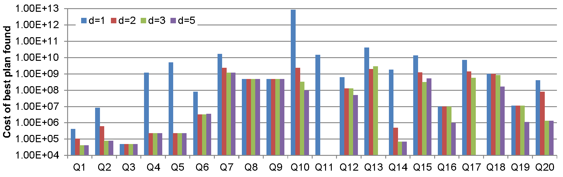Figure 1.a: Cost of the best plan with varying d

Clearly, in most cases, the largest cost reduction is achieved when incrementing d from 1 to 2, with a gain of 2 orders of magni- tude in half of the cases. Increasing d beyond 2 pays off mainly for queries relying some limited access relations, requiring an important reasoning effort to be inferred accessible.

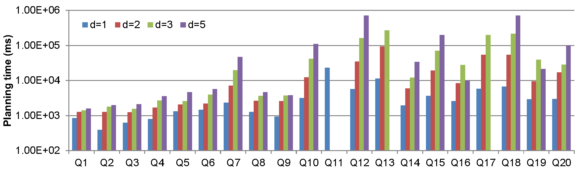Figure 1.b: Planning times with varying d

For all but one query, planning time is a few seconds for d=1, then increases by 1 to 2 orders of magnitude as d reaches 5. One outlier, Q₁₁, is our most demanding query. It has 8 atoms and triggers many constraints, leading to an initial chase with 22 atoms. For Q₁₁, planning with d=1 took 26 seconds, and increasing d to 2 caused the planner to time out (denoted by empty bars).

Overall however, setting d to 2 by default yields a very good cost reduction with a minor penalty on planning time.

Answerability

The next experiment investigates the benefits of constraint- awareness in the presence of access restrictions: how often our approach can find plans where a constraint-unaware optimizer will not find any, and how often it will find better plans than a constraint- unaware optimizer. We tested this by disabling integrity constraint in the reasoner. Accessibility axioms are still used, yielding an optimizer that finds the optimal plan that obeys the access methods, in the absence of constraints. In this experiment, we used S_default. We report the cost of the best plans found in Figure 2.a and the corresponding planning times in Figure 2.b. The red, hatch-patterned bars denote the constraint-oblivious cases, i.e. those for which integrity constraints were not taken into account. The blue bars correspond to cases where constraints were not taken into account. In both cases, we focused on the space of left-deep plans. For constraint-oblivious cases, we ran the search for left-deep plans exhaustively. The search space being much larger in the constraint-aware cases, we employed the priority ordering heuristic described above to ensure completion within the 15 minutes limit.

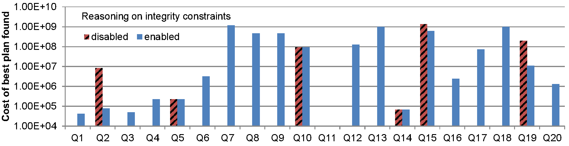Figure 2.a: Cost of the best plan with and without reasoning enabled.

The first observation one can make from these results is that even minor restrictions, such as those imposed on S_default, can render most of our queries unanswerable (missing red bars in Figure 2.a): only six queries turn out to be answerable. Moreover, for half of the queries that were answerable, the cost of plans was significantly reduced by enabling constraints.

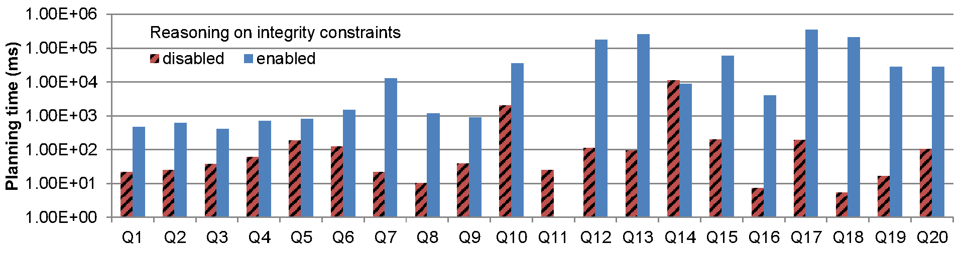Figure 2.b: Planning time with and without reasoning enabled.

However, as Figure 2.b shows, reasoning over constraints account comes at a price, as it requires to search through a much larger search space. In one instance, Q₁₈, planning time increased by 5 orders of magnitude. For Q₁ to Q₁₀ however, the penalty on planning times is mild, around 1 to 2 orders of magnitude, with an overall planning still under 1 second.

Impact of bushiness

Our implementation includes a "bushiness" parameter, which controls how many nested bushy joins are considered in proof and plan search. To test the impact of this parameter on plans costs, we use S_CP, for which 15 of our queries do not have any Cartesian products-free left-deep plan. One query, Q₆, becomes unanswerable in this schema.

Figure 3.a and 3.b show a comparison of the cost of the best plans found and the planning times respectively. In these figures, Bushy corresponds to our own bushiness-friendly algorithm.

In order to exhaustively search the space of plans and to see the impact of bushy search in isolation, these experiments were run without the distance-based heuristic. We allocated a 1h limit to the planner. Our bushy search looks for left-deep plans as an initialization phase, and thus most of the time it finds a plan at least as good as the best left-deep plan, if given the time to complete this initialization. However, our domination relation is an approximation of hereditary cost domination, and this approximation may remove subplans that can lead to optimal left-deep plans.

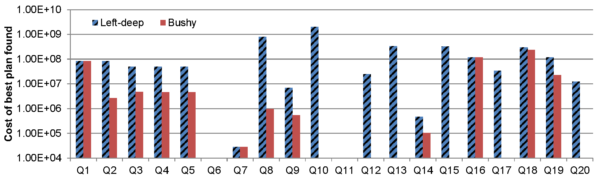Figure 3.a: Comparison of cost between left-deep and bushy plans.

The results show that allowing for bushy plans can lead to large improvements in cost. For two thirds of our queries, the planner managed to find plans within the allocated time. Moreover, searching for bushy plans pays off with a cost reduction of about one order of magnitude in half of those cases, while other plans were similar to the best left-deep ones.

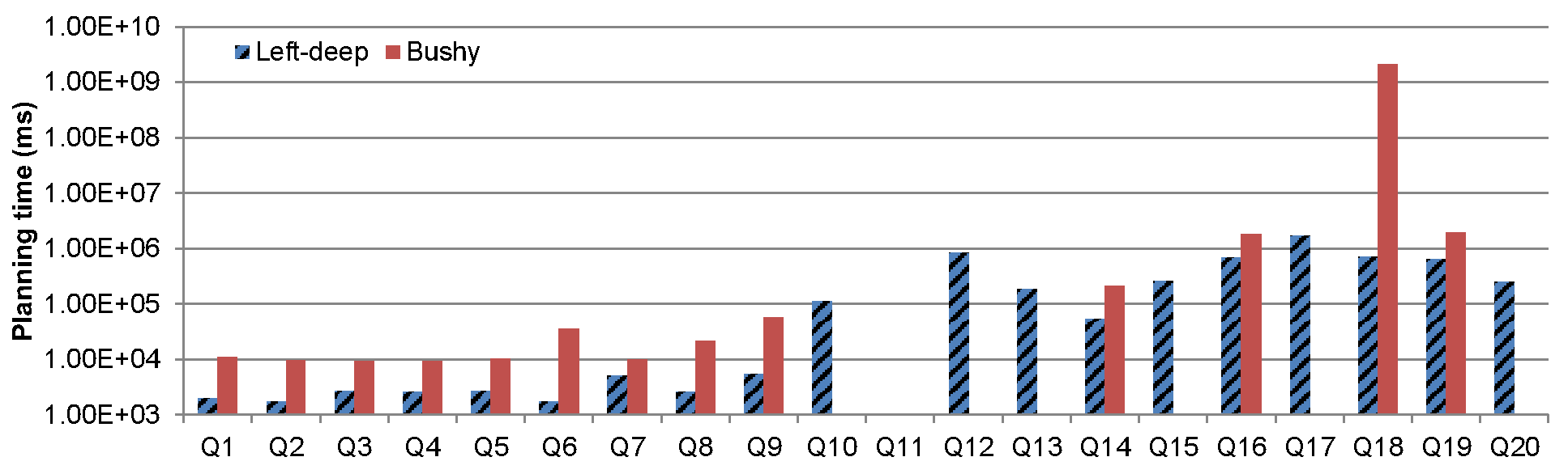Figure 3.b: Comparison of planning time for left-deep vs. bushy plans.

However, our current bushy search is still quite expensive, often leading to long planning times, reflecting the intrinsic combinatorial difficulty in searching for bushy plans in queries that when, expanded by constraints, may have >10 atoms. For the seven remaining answerable queries, the search for bushy plans times out without yielding any solution. This was partially related to the fact that the experiment did not apply the distance-based heuristic. Under this setting, even a left-deep plan could not be found for Q₁₁, our most expensive query. All other queries for which the planner timed out all use the lineitem relation. In our schema, this relation only has limited access and is 3 steps away from any free access relation in the dependency graph. Therefore, a large reasoning effort is required before lineitem is determined to be accessible, an effort that is compounded when bushy search is employed.

Impact of join ordering

Our last experiment compares the plans found by our system with those found by a minimal-rewriting approach, such as the chase and backchase. We mimicked the minimal-rewriting query-based approach (MR below) simply by setting our cost function to be the number of atoms, and then randomly re-ordering the atoms in the resulting plan. Note that, in cases where MR found multiple minimal rewritings, we randomly chose one of them. In evaluating our system and the minimal-rewriting-based one, we used the PostgreSQL plan analyser tool EXPLAIN to evaluate the cost. As our system produces physical plans, in contrast to MR which returns logical rewritings, we translated the plans or rewriting found by our system and MR, respectively, to SQL queries, which were subsequently supplied to PostgreSQL for analysis. In this experiment, our system was restricted to search for left-deep plans.

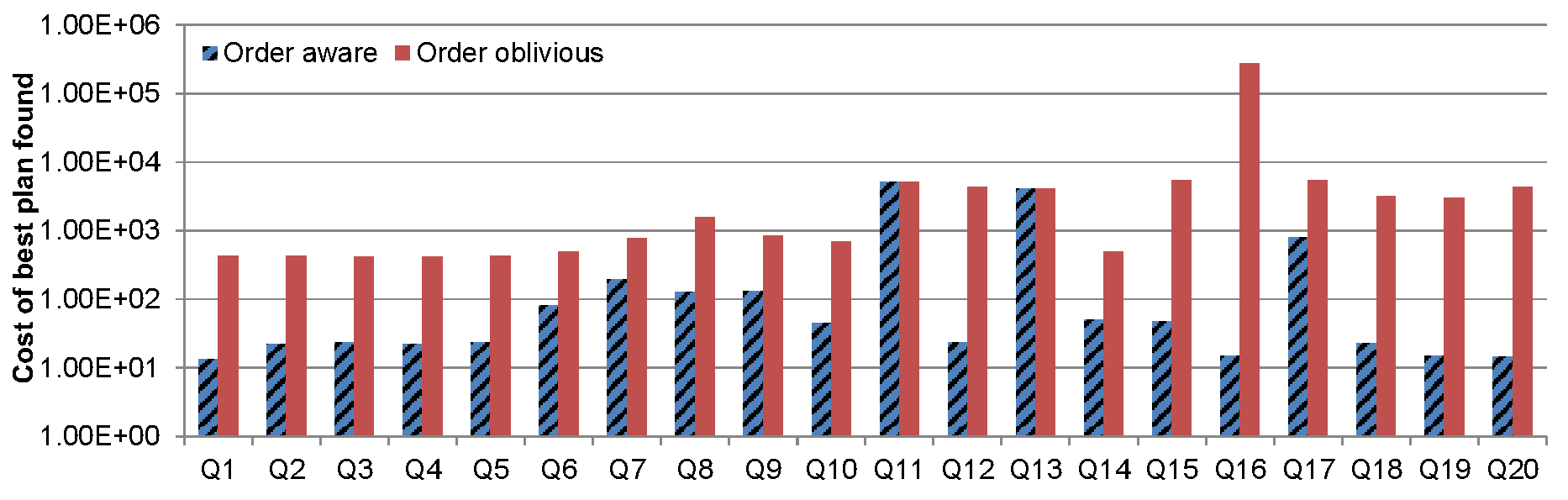Figure 4.a: Cost of the best plan found for order-aware vs. order-oblivious planning

The results are presented in Figure 4.a. In most of the cases, we can observe improvements of several orders of magnitude. For example, Q₂ asks for the manufactures of the parts whose available quantity is 10 units:

{<manufacture> | partsupp(partkey, partname, 10, ...) ∧ part(partkey, manufacture, ...)}

Some of the input-free-access views that our schema has are part_partsupp, supplier_partsupp, and nation_supplier, which are the natural joins of the corresponding tables. It is clear that our query can be directly answered by accessing the part_partsupp view. This is actually the minimal rewriting returned by MR. For this rewriting, PostgreSQL produces a physical plan that, first, performs a sequential scan on part_partsupp and, second, filters out the tuples with available quantity = 10. The total cost of these operations is estimated at 433.00. However, we could answer that query approximately 20 times faster by first accessing the nation_supplier view, then the supplier_partsupp view and finally the part_partsupp view. In particular, the physical plan that PostgreSQL produces joins the tuples of nation_supplier with the ones of supplier_partsupp, after performing, first, a se- quential scan on nation_supplier and, second, an indexed scan on supplier_partsupp filtering out the tuples with available quantity <> 10. The total cost of the above operations is estimated at 13.69. As a final step, it joins the previously derived tuples with the ones acquired after performing an indexed scan on part_partsupp and filtering out the tuples with available quantity <> 10. The overall cost is estimated at 22.13.

Note that all of our algorithms optimize based on cost estimates, either through the simple textbook cost function or (in the order-aware vs. order-oblivious experment) via the cost function of Postgres. We do not claim that our cost estimates are accurate. Furthermore, in the last experiment, we found that even the estimates of PostgreSQL were quite far from actual runtimes. To exemplify this, we give the corresponding runtimes for the order-aware and order-oblivious experiments below.

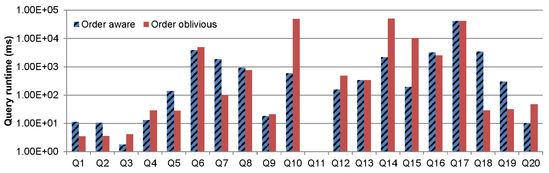Figure 4.b: Query runtimes for order-aware vs. order-oblivious plans